Friday, 26 December 2014

I wanted to drop all my temp tables at the top of a large SELECT statement and already had a query to drop a Named temp-table …
IF OBJECT_ID('tempdb..#Temp2') IS NOT NULL DROP TABLE #Temp2
… so just needed to make that dynamic. Looking at the temp tables …
select * from tempdb.sys.objects where name like '#%'
… I noticed all mine had a bunch of underscores and a GUID appended to the name. And the GUID always contained atleast 5 zero’s. So I was able to filter out just mine with
select name from tempdb.sys.objects where name like '#000%'
… and paste that into a while loop to drop them …
--first drop all temp tables
IF OBJECT_ID('temptables') IS NOT NULL DROP TABLE temptables
select name into temptables from tempdb.sys.objects where name like '#000%'

declare @table varchar(max), @cmd varchar(max)
while (select count(*) from temptables) > 0
begin
 set @table = (select top 1 name from temptables)
 set @cmd = 'IF OBJECT_ID(''tempdb..' + @table + ''') IS NOT NULL DROP TABLE ' + @table
 exec(@cmd)
 delete from temptables where name = @table
end

DROP TABLE temptables
By initially creating a list and then working through it deleting the temp-table and its entry in the list, I ensured there would be no endless looping should it try (and fail) to drop a temp-table I don’t have permissions on

Tuesday, 23 December 2014


How to create, find and eliminate deadlocks


Deadlocks are typically encountered in high-load scenarios or in complex concurrent transactions. And the worst part is, you probably won’t see them until you’re live in production. Luckily, finding and solving deadlock issues isn’t as complicated as it may sound. All it takes is a bit of logging and patience, along with some basic know-how of how locking mechanisms work in SQL Server.

What’s a deadlock?

A deadlock occurs when two processes are waiting for the same resources – and both of these processes are waiting for the other to finish.
Imagine the following example of a banking database: Alice and Bob have bank accounts, and they want to send each other money. The process of sending money from one account to another involves two bookings that have to be atomic, i.e. run in a transaction. Because if the server or network connection fail after only half the operation has been completed, the balances would be off, and somebody would probably end up having a pretty bad day.
Alice starts off by moving $1000 to Bob’s account: (process 1)
BEGIN TRANSACTION;

   UPDATE banking.accounts
   SET balance=balance-1000
   WHERE account='Alice';

   UPDATE banking.accounts
   SET balance=balance+1000
   WHERE account='Bob';

COMMIT TRANSACTION;
But what if Bob, only a millisecond after Alice, clicks the “Send” button on his Internet banking web page, to send $500 to Alice? The code would look like this: (process 2)
BEGIN TRANSACTION;

   UPDATE banking.accounts
   SET balance=balance-500
   WHERE account='Bob';

   UPDATE banking.accounts
   SET balance=balance+500
   WHERE account='Alice';

COMMIT TRANSACTION;
Here’s a timeline of what happens:
  • Alice takes $1000 from her account (process 1). This creates a lock on her account (so nobody else can change the balance, in case we need to roll back the transaction later).
  • Bob takes $500 from his account (process 2), placing a lock on his account.
  • Alice (process 1) is now waiting for the Bob (process 2) to commit his transaction, so the lock on Bob’s account is released, before she can complete the transfer.
  • At the same time, Bob (process 2) is waiting for Alice (process 1) to commit her transaction.
In the end, both Alice and Bob are waiting for each other to complete their respective transactions, and they could technically wait forever. This is where the deadlock monitor, a system process in SQL Server, steps in an kills (rolls back) the process that has done the least amount of work. The killed process, known as the deadlock victim, receives the following error message:
Msg 1205, Level 13, State 51, Line 1
Transaction (Process ID 73) was deadlocked on lock resources with
       another process and has been chosen as the deadlock victim.
       Rerun the transaction.
In the example above, the objects of the deadlock are two rows in the same table, but the object of a deadlock can be a number of different things – tables, pages, rows, schemas, locks, even chunks of memory or worker threads. However, wer’re going to limit our scope to the most common kind, database objects.

Using SQL Server Profiler to identify deadlocks

A trace in SQL Server Profiler can give you details as to what objects are deadlocked. Start off from a blank template, then, under “Locks”, check the “Deadlock graph”, “Lock: Deadlock” and “Lock: Deadlock Chain” events.
You can run this trace interactively (with the Profiler window open) or in the background, as a server-side trace if you want to keep logging for a longer time. Just remember to stop your server-side trace once you’re done. A lot of people will tell you that a long-running trace takes a lot more resources if it runs interactively in Profiler than as a background trace, but I haven’t verified this myself.
Once you find deadlock events, you can view the dependency graph in Profiler to find out which objects were involved. From that, you can hopefully deduce what procedure or queries to tune. If you can’t, simply add those events as well, but be aware that your trace log can fill up pretty fast if you do.

How to avoid deadlocks

As you’ll understand by now, deadlocks are naturally occurring in databases, and the more transactions you run through it, the more likely a deadlock is to happen. So mostly, there is no sure-fire way of completely eliminating deadlocks. The best you can do is a kind of “harm reduction”, where you a) minimize the number of deadlocks, and b) handle those that happen, by trapping deadlocks and rerunning the transactions.

Guidelines for minimizing the number of deadlocks

In my personal order of preference:
  • Deadlocks (nearly) always happen in SQL transactions. Time is a factor, so keep transactions as short as possible. Optimize indexes for performance on critical tables. And never, ever, leave an uncommitted transaction waiting for user input.
  • For all operations that are atomic, keep the size of the operation to an absolute minimum, as far as your situation allows for.
  • Use locking hints to place more specific locks. Lock all your resources as quickly as possible.
  • Make sure all your code places locks in the same order.
  • Try different isolation levels.

How to handle a deadlock

Deadlocks can be trapped using a TRY-CATCH block. If your transaction is deadlocked, it is rolled back to the point of the BEGIN TRANSACTION statement.

Locking order

If you always lock objects in the same order, you will significantly reduce the risk of those objects being part of a deadlock. To look at the banking example above, if we always make the transfers in the alphabetical order of the account holder’s name, here’s how Bob’s transfer (process 2) would have looked:
BEGIN TRANSACTION;

   -- 'Alice'<'Bob', so her account goes first:
   UPDATE banking.accounts
   SET balance=balance+500
   WHERE account='Alice';

   UPDATE banking.accounts
   SET balance=balance-500
   WHERE account='Bob';

COMMIT TRANSACTION;
With this new setup, let’s go through the timeline again:
  • Alice takes $1000 from her account (process 1). This creates a lock on her account.
  • Bob (process2) waits for Alice.
  • Alice adds $1000 to Bob’s account (process 1).
  • Alice (process 1) commits her transaction.
  • Bob (process 2) now adds $500 to Alice’s account.
  • Bob (process 2) removes $500 from his account.
  • Bob commits his transaction.

Locking hints

Using locking hints, it’s possible to tell SQL Server what kind of locks to place. This is practical when you’re handling lock escalation. Lock escalation occurs when a lock is converted, for instance from a shared lock to an update or exclusive lock. Lock escalations happen all the time, and mostly, SQL Server gets it right. However, it can only guess what you want to accomplish, so you can help it along by explicitly specifying what types of locks and what granularity you want.
Depending on your query, an aggressive lock (exclusive table or schema lock) may work better or worse than a relaxed strategy (intent shared, row lock). The best strategy is very dependent on how your transaction looks and how much work it does.
Locking hints are defined with the tables in a query:
...
FROM dbo.table_a AS a WITH (TABLOCKX, HOLDLOCK)
LEFT JOIN dbo.table_b AS b WITH (NOLOCK) ON ...
Here are some common locking hints
  • TABLOCK and TABLOCKX: Table lock and exclusive table lock. One lock is placed on the entire table.
  • PAGLOCK: Places a page lock. A page is an 8 kB unit of storage.
  • ROWLOCK: Locks individual rows. Very fine-grained, should only be used on very small quantities of data.
  • UPDLOCK: Update lock, allows other processes to view locked data, but not change it.
  • NOLOCK: Applies to SELECT statements only. Does not place any lock and does not honor any existing locks from other processes.
A locking hint-based solution to the deadlock example above could be placing initial locks on both rows before performing the two updates:
BEGIN TRANSACTION;

   --- Place a rowlock on each of the two rows and hold these
   --- locks for the remainder of the transaction.
   SET @dummy=SUM(balance)
   FROM banking.accounts WITH (ROWLOCK, HOLDLOCK)
   WHERE account IN ('Alice', 'Bob')
   UPDATE banking.accounts
   SET balance=balance-1000
   WHERE account='Alice';

   UPDATE banking.accounts
   SET balance=balance+1000
   WHERE account='Bob';

COMMIT TRANSACTION;
This way, both accounts are locked the instant we start the procedure. The HOLDLOCK hint makes sure that the two locks are held until we commit or roll back the transaction.

Deadlock priority

Normally, when a deadlock occurs, the transaction that has accomplished the least amount of work is the one that is chosen as the deadlock victim, i.e. rolled back with an error message.
However, you can assign different priorities to different transactions, depending on what they do or how critical they are.
SET DEADLOCK_PRIORITY HIGH
Valid parameters are LOW, NORMAL, HIGH, or numeric values between -10 and 10. A lower number or LOW means that there is a higher probability that the transaction will be selected as the victim in a deadlock.

Rebuilding a transaction log file


The database’s transaction log file contains, like the name implies, a log of all the transactions happening in the database. If you’ve set your database to the “simple” recovery model, the log is truncated (emptied) at every checkpoint (more or less all the time). In “bulk logged” or “full” recovery model, you’ll have to truncate the log files yourself, by performing a transaction log backup.
So because of this, the log file has to stay in sync with the rest of the database at all times. But what do you do if your log file is lost or corrupted? Luckily, there’s a simple way to recover it.

I’ve discovered to ways to remedy this problem, for two different scenarios.

The simple option: Attaching a clean database

If your database was shut down cleanly and you have all the database files (except the log file, of course), you can just attach the database using the CREATE DATABASE statement with FOR ATTACH_REBUILD_LOG.
It’ll look something like this:
CREATE DATABASE DatabaseNameHere
ON (FILENAME='D:\File1.mdf'),
   (FILENAME='D:\File2.ndf'),
   (FILENAME='D:\File3.ndf'),
   (FILENAME='D:\File4.ndf')
FOR ATTACH_REBUILD_LOG;
This basically attaches the database from the MDF/NDF files, and creates a blank, 1 MB large log file from scratch in the default log directory of your server. This is by far the easiest and least risky way to recreate a new log file.
This will of course break the backup chain, but then again, if you’ve lost your log file there’s really not much else you could do anyway.

The tricky option: database is suspect

In some situations, a corrupt log file will render the database “suspect”. First off, change the database mode to “emergency” and to single user mode using the following script. I’ve added “read-write” as well, in case the database is set as read-only:
ALTER DATABASE databaseName SET EMERGENCY;
ALTER DATABASE databaseName SET SINGLE_USER;
ALTER DATABASE databaseName SET READ_WRITE;
If the database is now in single-user, emergency mode, you can run a DBCC command on it. The following DBCC operation does not only create a new log file, but also checks the database for consistency errors, so it may take a while to run, depending on the size of your database.
DBCC CHECKDB (databaseName, REPAIR_ALLOW_DATA_LOSS);
With a little bit of luck, the operation will succeed, and your heart rate and blood pressure will go down a notch. Now, all you have to do is set the database back online and for multi-user use.
ALTER DATABASE databaseName SET MULTI_USER;
ALTER DATABASE databaseName SET ONLINE;
I don’t really have loads of experience of crashing log files, though a… uhm… friend of mine managed to lose a log file once. I’ve tried the solution above, and it worked for me once. Your mileage may vary, though.
Best of luck, anyway!

Introduction to partitioning


Partitioning is not only a great way to improve performance in large tables, but you can also use it to manage the physical storage of different chunks of data without keeping it in different tables.

First off, to use partitioning on SQL Server, you need the Enterprise Edition, which comes with a hefty price tag and as such is really only suited for more demanding setups.

How partitioning works

Partitioning data means that you split the physical storage of it into different filegroups (which in turn typically means different physical storage locations). This creates a number of performance benefits, because although the table (for instance) is still visible as one table with data, in actual fact, it is stored as a number of tables physically. And smaller tables means better performance.
You can partition a table, a heap or an index. When you partition a table (with a clustered index) it’s actually the clustered index, which makes up the physical storage of the table, that is being partitioned.
Some of the benefits of partitioning your data are obvious, other not:
  • Using partition elimination, SQL Server can query a single partition to increase performance.
  • You can apply different data compression to different partitions, depending on your needs.
  • Data that is frequently updated can reside on storage with good write performance, while older data that typically doesn’t change can be stored on disks with better read performance.
  • Self-joins (actually, “equi-joins”) can be performed more efficiently because two partitions can be treated as separate tables.
  • Partitioned data allows for partition switching – an advanced and very, very efficient way to move entire partitions of data between two identical tables/partitions.

Aligned indexes

When you have a partitioned table, you can partition the table’s non-clustered indexes as well. This does not happen automatically, and you can choose different partition schemes for the table and its indexes independently of each other.
However, if you choose a partition scheme for a non-clustered indexes that is essentially equivalent to that of the table, that index is referred to as being “aligned” to its table, which brings a few performance advantages which I won’t go into here, mostly related to switching or moving data in and out of partitions.

Creating a partition function

The first thing you need is a partition function. This is basically the definition of which rows end up in which partition.


--- Create the partition function:


CREATE PARTITION FUNCTION fn_part_left(int) AS RANGE LEFT FOR VALUES (100, 110, 120, 130);
The “boundary values” for this partition function are 100, 110, 120 and 130. This means that these values are the lower and upper boundaries of each partition.
A partition function can either be RANGE LEFT or RANGE RIGHT. Whether a partition function is “left” or “right” defines on which partition to store values that are exactly equal to a boundary value:
value        RANGE LEFT partition   RANGE RIGHT partition
98             1                      1
99             1                      1
100            1                      2
101            2                      2
102            2                      2
...
128            4                      4
129            4                      4
130            4                      5
131            5                      5
132            5                      5
The boundary values of the example partitions have been highlighted in red above.
For a RANGE LEFT partition function, the first partition will include values up to and including the first boundary value and the last partition will include values above the last boundary value.
For a RANGE RIGHT partition function, on the other hand, the first partition will include values below the first boundary value and the last partition will include values starting at the last boundary value.


To test which partition a given value would end up in, you can use the special $PARTITION function, like this:


SELECT $PARTITION.fn_part_left(123);


.. where fn_part_left, in this case, is the partition function, and 123 is the value we want to test. You can also prefix $PARTITION with a specific database name.
SELECT databaseName.$PARTITION.partFunction(123);

Creating a partition scheme

Second, you need a partition scheme which defines which filegroups are used for each partition in the partition function.
--- Create the partition scheme:
CREATE PARTITION SCHEME ps_part_left AS
PARTITION fn_part_left TO
    ([GROUP_A], [GROUP_B], [GROUP_C], [GROUP_A], [GROUP_B]);
Remember, you need one more partition than the number of partition boundaries. So if you have four boundaries, that means you need five partitions. If you want to, you can define all the partitions on the same filegroup using the ALL keyword.
--- Create the partition scheme,
--- all partitions on the same filegroup:
CREATE PARTITION SCHEME ps_part_left AS
PARTITION fn_part_left ALL TO ([PRIMARY]);

Creating a partitioned table or index

When creating tables and indexes, you declare the partition scheme and partitioning column where you would otherwise declare a filegroup, using the ON keyword:
--- Create a table on the partition scheme:
CREATE TABLE dbo.tbl_part_left (
     i      int NOT NULL,
     PRIMARY KEY CLUSTERED (i)
) ON ps_part_left(i);

Partitioning an existing table or index

An existing index or an existing table with a clustered index can be moved to a partition scheme using CREATE INDEX with DROP_EXISTING.
--- Create a standard, unpartitioned table:
CREATE TABLE dbo.tbl_unpart (
    i          int NOT NULL,
    CONSTRAINT PK_tbl_unpart PRIMARY KEY CLUSTERED (i)
) ON [PRIMARY];

--- Populate the table with some example data:
INSERT INTO dbo.tbl_unpart (i)
VALUES (98), (99), (100), (101), (102),
       (103), (104), (105), (106), (107),
       (108), (109), (110), (111), (112),
       (130), (131), (132), (133);

--- Move the existing table to a partition scheme using
--- CREATE INDEX with DROP_EXISTING:
CREATE UNIQUE CLUSTERED INDEX PK_tbl_unpart ON dbo.tbl_unpart (i)
        WITH (DROP_EXISTING=ON)
    ON ps_part_left(i);
This was a very short introduction to partitioning, but as you understand, it’s a fairly deep topic, and there’s lots of room for discussions like partition switching, merging, compression, etc. Stay tuned for more further on!

Shrinking tempdb without restarting SQL Server


Ok, so even if you’re a seasoned veteran T-SQL coder, at some time you will write a query that runs away and supersizes the tempdb database. This, in turn, might fill up your disk and cause other server-related problems for you. At that point, you may find out the hard way that shrinking tempdb isn’t like shrinking any other database.


Here are some tricks that I’ve tried successfully – but bear in mind that your mileage may vary.

Tempdb stores temporary tables as well as a lot of temporary (cached) information used to speed up queries and stored procedures. For the best chances in shrinking tempdb, we’re going to clear these different caches (except for the temp tables, which you should drop manually).

First off, the easy way out

It’s worth mentioning. If you’re not running a production-like environment, your best bet is to restart the SQL Server service. This will return tempdb to its default size, and you won’t have to worry about all the potential pitfalls of this article. But since you’re reading this, chances are you can’t just restart the server. So here goes:
Warning: These operations remove all kinds of caches, which will impact server performance to some degree until they’ve been rebuilt by the SQL Server. Don’t do this stuff unless absolutely neccessary.

DBCC DROPCLEANBUFFERS

Clears the clean buffers. This will flush cached indexes and data pages. You may want to run a CHECKPOINT command first, in order to flush everything to disk.
CHECKPOINT;
GO
DBCC DROPCLEANBUFFERS;
GO

DBCC FREEPROCCACHE

Clears the procedure cache, which may free up some space in tempdb, although at the expense of your cached execution plans, which will need to be rebuilt the next time. This means that ad-hoc queries and stored procedures will have to recompile the next time you run them. Although this happens automatically, you may notice a significant performance decrease the first few times you run your procedures.
DBCC FREEPROCCACHE;
GO

DBCC FREESYSTEMCACHE

This operation is similar to FREEPROCCACHE, except it affects other types of caches.
DBCC FREESYSTEMCACHE ('ALL');
GO

DBCC FREESESSIONCACHE

Flushes the distributed query connection cache. This has to do with distributed queries (queries between servers), but I’m really not sure how much space they actually take up in tempdb.
DBCC FREESESSIONCACHE;
GO

.. and finally, DBCC SHRINKFILE

DBCC SHRINKFILE is the same tool used to shrink any database file, in tempdb or other databases. This is the step that actually frees the unallocated space from the database file.


Warning: Make sure you don’t have any open transactions when running DBCC SHRINKFILE. Open transactions may cause the DBCC operation to fail, and possibly corrupt your tempdb!
DBCC SHRINKFILE (TEMPDEV, 20480);   --- New file size in MB
GO


Don’t set the new size too low! Make a realistic estimate of the largest “normal” size that tempdb will assume during normal day-to-day operation.
That’s it. If everything works the way it should, you should now be able to verify the new size of tempdb.

A word about shrinking database files

Best practice is to try to minimize the use of file or database shrinking as much as possible. Whenever you shrink a database file and it re-grows later on, you are potentially creating fragmentation on your physical storage medium. This is because the sectors that the file used to occupy may now very well be occupied by other information (just a few bytes are enough). When SQL Server wants to grow that database file, the newly added portion of the file will need to be placed elsewhere on the disk, thus creating fragmentation.


The number one mortal sin in this context is “autoshrink“, because it may very well add to the drive fragmentation every time it runs, which could be very frequently.
As a rule of thumb, never ever autoshrink a database. And try to be very restrictive when it comes to shrinking databases or files in general, unless it’s a one-off operation to fix the aftermath of a runaway query.

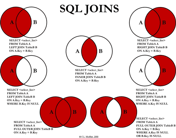
SQL joins illustrated 


Enjoy!
Reading a query plan


Knowing how to read a query plan is absolutely key to optimizing SQL Server query performance. The query plan tells you how SQL Server goes about running your query, including what indexes are used (and how), what join strategies are applied and a lot of other information. If you can read the query plan, you can make the appropriate changes to indexes, query hints, join conditions, etc to tune your workload for optimum performance.

How to view a query plan

You can show an estimated query plan by selecting the query you want to evaluate and press Ctrl+L. This will set the SHOWPLAN flag in SQL Server, so the execution of the query is limited to just displaying the query plan, not actually executing the query.
The other way is to enable “Include actual query plan” (press Ctrl+M to toggle). The difference between these two is that the actual query plan is displayed as the query runs. The estimated query plan is, like the name implies, just an estimate. In my opinion, the two rarely differ significantly.
Here’s an example of how your query plan might look.

Queryplan for HumanResources.vEmployee

The flow of it

Query plans are read from right-to-left; that is, each table or index that is collected along the way is a “leaf” node, all the way out to the right, and the final result of the operation is the top-left node. In the example plan above, you can see that we’re joining 7 different tables into one big SELECT query.
It’s important to understand that while T-SQL is merely a language that describes what you want to do with your query, the actual query plan may actually differ significantly from how you write the query. The reason for this is that the SQL Server optimizer normally does a very good job in finding the most efficient method to solve the task at hand, but that method may not follow for instance the join order or methods that you imagined. It all comes down to how the data is physically arranged in the database.

Indexes and statistics

The primary help for the query optimizer in this task are the different indexes and statistics that exist on the different objects that are referenced in the query. For this reason, making sure that tables are well-indexed and that their statistics are up-to-date can dramatically improve your query performance.

Common query plan operators

Here’s a fairly common selection of operators you will probably encounter in query plans:
Clustered index seek Clustered index seek, Index seek index seek
An index seek is where the server looks for a single value or a closed interval of values. Unless you want to return the entire index/table, a seek is generally preferrable to a scan (see below).
Clustered index scan Clustered index scan, Index scan index scan
An index scan occurs when it’s not possible to “seek” a value in the index, for instance because you’re using a wildcard condition. It is also applied when you deliberately want to make use of the entire index or (clustered) table.
Table scan Table scanIf this operator turns up, you’ve forgotten to create a clustered index to your table. It goes through the entire table, top-to-bottom, which is resource-consuming and results in very poor performance and takes a heavy toll on the I/O. A table scan only happens when there is no suitable index available to complete the query.
Nested loops Nested loops
Nested loops is a way to JOIN two tables. This method is mostly practical when one table is considerably larger than the other. For each row in the “outer” table, it loops through the “inner” table.
Merge join Merge join
A merge join is the single most optimal join method from a performance standpoint, but in order to achieve it, the key columns of the two data sets to be joined need to match perfectly with regard to data types and sort orders.
Hash match Hash match, hash join
This is the JOIN method applied if a nested loop or merge join is not feasible. It uses internal hash tables to join two data sets.
Filter Filter
The filter operator most closely resembles the WHERE or HAVING clauses, where these operations cannot be performed directly on the index or table.
Constant scan Constant scan
Represents the use of constants, without the need to retrieve any value from an actual index or table, for instance
SELECT 123 AS my_integer;
Compute scalar Compute scalar
Any scalar calculation performed, for example arithmetic operations, string functions, etc.
Sort Sort
Sorting the dataset can be performed at the end of the query in order to comply with an ORDER BY directive, or for instance before a JOIN operator in order to prepare the data set for a more optimized join method.

Tooltip information

If you hover over a node in the query plan, you’ll see a lot of detailed information about each node. The most important ones to look for are the estimated I/O and CPU costs (how much disk input/output workload and computing power respectively that the step will consume), as well as the subtree cost.
Also, take a look at the output list and/or predicates, at the bottom of the tooltip. They provide more detail about columns are used in a join operator, what columns is output from an index scan, etc.

More details

Again, this is but a selection of common query plan operators that you’re likely to encounter. There are a lot more operators, with more detailed descriptions, available on MSDN. A deeper discussion on the performance aspects and requirements of different JOIN and indexing stragies will be the topic of a separate post. Stay tuned.